Class 11: Poisoning

18 Apr, 2018 · by Team Gibbon

This week we discussed poisoning attacks, which differ from previously-discussed attacks in a key way. Instead of finding test instances that the target model misclassifies, a poisoning attack adds “poisoned” instances to the training set, introducing new errors into the model. Below are three papers which discuss interesting work happening in this field.

Poison Frogs!

Ali Shafahi, W. Ronny Huang, Mahyar Najibi, Octavian Suciu, Christoph Studer, Tudor Dumitras, and Tom Goldstein. Poison Frogs! Targeted Clean-Label Poisoning Attacks on Neural Networks. April 2018. arXiv e-print [PDF]

A Simple Clean Label Attack

The paper presents a novel clean-label attack, which restricts the attacker to injecting correctly-classified examples into the victim’s training set. The goal of the attacker is to make the model misclassify a “target” instance, specifically to the same class as some chosen “base” instance. The attack is executed by subtly changing the base instance to display features of the target; this is illustrated in Figure (a) below. Figure (b) shows a simple diagram of the intended effect on the model’s decision boundary. When the model trains, it hopefully overfits on the poisoned instance, thereby allowing the target to be classified incorrectly. The major benefit of this approach is that it is difficult for the victim to detect: since the poisoned data is still labeled correctly, the model’s test accuracy should not change.

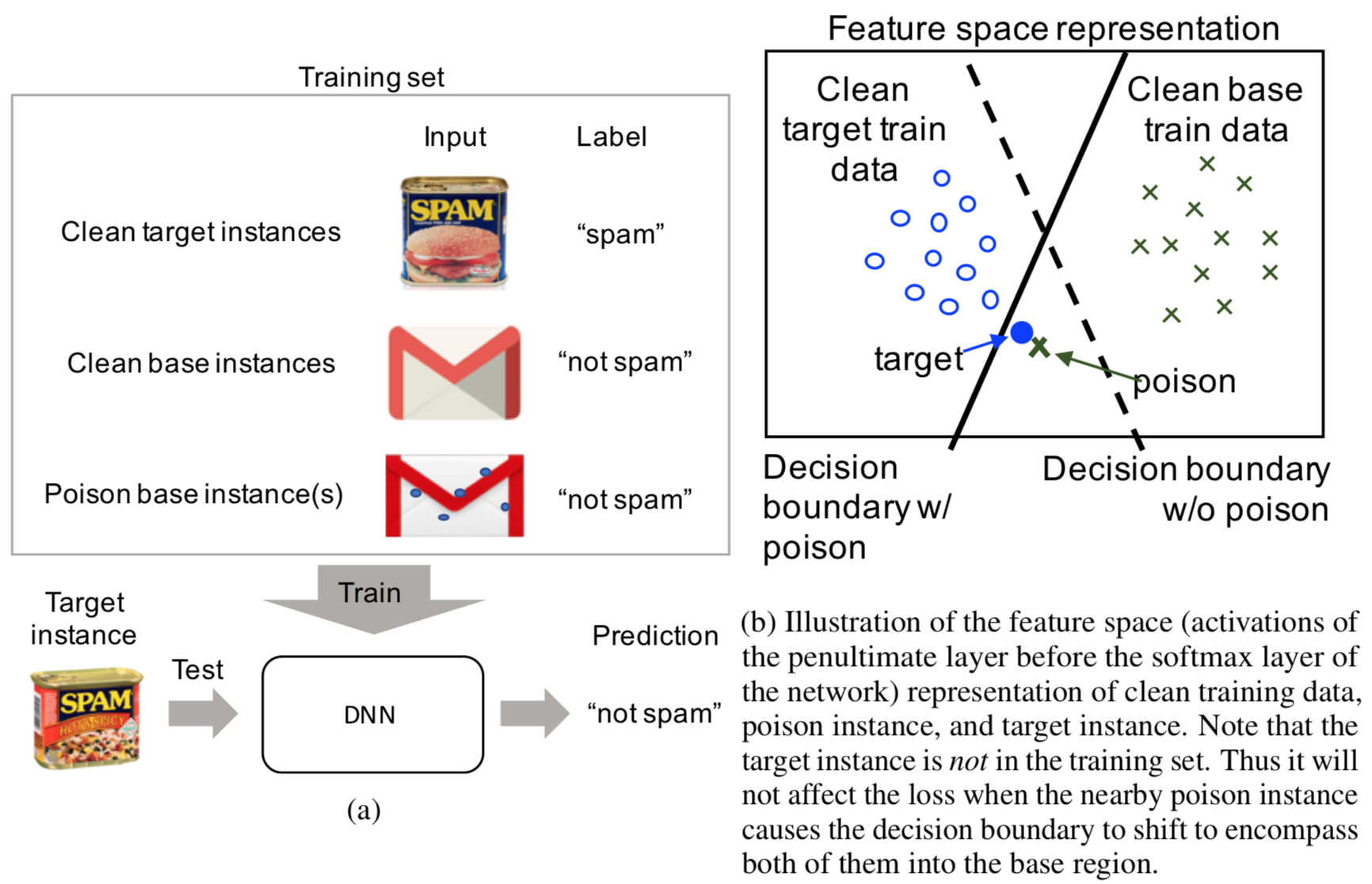
In more formal language, the clean-label attack does this: given a target instance $t$ and a base instance $b$, create a poisoned instance $p$ such that

$p$ is humanly-indistinguishable from $b$ (and is classified the same), and
the model, after training on a data set that includes $p$, misclassifies $t$ to be in the same class as $b$.

The equivalent optimization problem is

where $\beta$ represents how closely $p$ resembles the base instance $b$. There is a simple algorithm for solving this optimization problem: alternate between “forward steps” to inch closer to $t$ and “backward steps” to stay close to $b$.

The clean-label attack works extremely well on transfer learning models, which contain a pre-trained feature extraction network hooked up to a trainable, final classification layer. As an example, the authors created an InceptionV3 model that classified images of dogs and fish. They were able to attack this model a 100% success rate by including just one poisoned image in each attack; furthermore, the target images were misclassified by the model with high confidence:

Watermarking Attack on End-to-End Training

The poisoning attack above is effective when the early feature extraction layers of a network are not retrained (as in transfer learning), but is not as effective when training end-to-end. The figure below shows this effect measured by the angular deviation of the decision boundary. The angular deviation is the angular difference between the decision boundary of a clean and poisoned network. A high angular deviation indicates the poisoning attack was strong, causing the decision boundary to significantly shift. We see that the poisoning attack we’ve discussed does not shift the decision boundary on end-to-end learning nearly as much as it does for transfer learning.

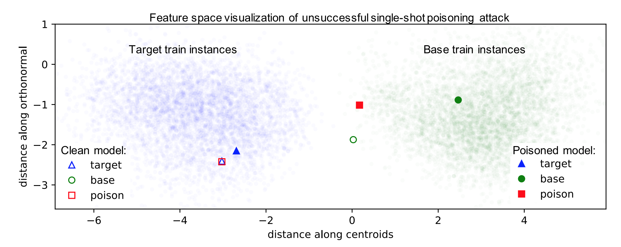
The figure below shows the feature space representations of the target, base, and poison instances in the context of their training data for a single-shot poisoning attack. The clean model shows the target and poison instance overlapping – this indicates the optimization algorithm to find a poison instance works. However, we see that retraining the network separates the poison and target instances and returns the poison instance to the base class.

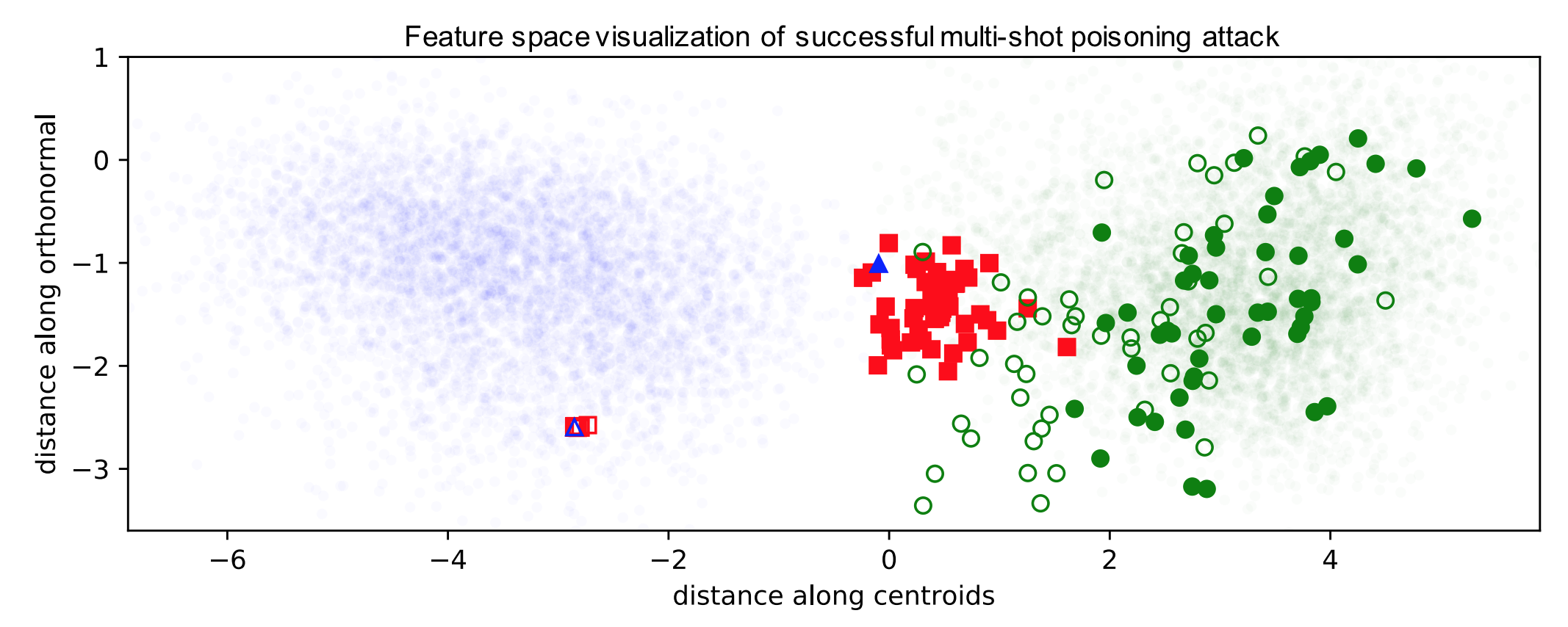
To fix this, the authors use a technique called watermarking. Watermaking blends additional features of the target instance into the poison instance in a way humans can’t notice. In particular, a low opacity watermark of the target instance is added to the poison instances. Watermarks are not noticeable to humans up to 30% opacity. The figure below shows how constructing 50 poison instances from 50 random base instances casuses the target instances to be pulled out of the target feature space into the base class feature space, resulting in incorrect classifications.

We see below 60 images of dogs with watermarks of birds at 30% opacity. These poison instances successfully cause a target image of a bird to get misclassified as a dog with end-to-end training.

The authors found that targeting outlier instances has a 17% higher success rate. Since these targets lie far from other training samples in their class, they are close to the decision boundary, and it is therefore easier to flip their class label. Additionally, the authors found that the attack success rate was higher when more poison instances were included in the retraining and when the watermark had a higher opacity.

Poisoning Regression Learning

Matthew Jagielski, Alina Oprea, Battista Biggio, Chang Liu, Cristina Nita-Rotaru and Bo Li. Manipulating Machine Learning: Poisoning Attacks and Countermeasures for Regression Learning. April 2018. arXiv e-print [PDF] (IEEE Symposium on Security and Privacy 2018)

It is well understood that machine learning models are easy to be manipulated by smart attackers. There are both test-time evasion attacks and training-time data poisoning attacks, so studying and understanding these potential risks is beneficial for the application of machine learning in security critical domains.

In this paper, the authors studied the specific problem of training a data poisoning attack on linear regression models and subsequently proposed an effective defensive strategy.

A linear regression is defined as

And the loss function being optimized during the training time is the mean-squared error (MSE), which is defined as:

MSE is used here as the result of linear regression and is a continuous value, while a traditional classification task outputs discrete categorical values. The term $\Omega(\mathbf{w})$ denotes the regularization terms. When we take different norms, it corresponds to different regularization functions. ($L$2-norm corresponds to ridge regression, $L$1-norm to LASSO regression, and Elastic-net Regression takes the linear combination of $L$1-norm and $L$2-norm).

Optimization-based Poisoning Attack

The attack aims to corrupt the machine learning in the training phase by introducing noisy training data points such that predictions at test time will be influenced. The author considered both the white-box and black-box attack. White-box attack means the attacker is aware of all the information including training dataset, feature values, training algorithm and trained parameters. In the black-box setting, the training dataset is assumed to be unknown. With all these described, we arrive at the following formulation regarding training data poisoning attack:

where $\mathbf{\theta}{p}^{*}$ is the model parameter obtained by training the model on poisoned training dataset. $D{tr}$ denotes unpoisoned training data, and $D_{p}$ are the poisoned training data, which typically takes around $10%$ of the clean training data. $W(D^{'},\mathbf{\theta}_{p}^{*})$ is the loss function defined on the test (or validation) dataset $D^{'}$, which is free from the poisoning attacks. (Sorry, can’t fix the mathjax typesetting for this paragraph; please check the original paper if confused.)

Note that this is a bilevel optimization problem and is different from the traditional optimization we know, in that the constraint itself is an optimization problem. Also, the parameter $\theta_{p}^{*}$ depends implicitly on the poisoned training dataset $D_{p}^{*}$.

To optimize the above problem with respect to a set of data points $D_{p}$, the approach is to optimize each instance $\mathbf{x}_{c}$ in the set $D_{p}$. With this, the authors apply gradient descent algorithms to find an optimal $\mathbf{x}_c$ that can maximize the loss function $W(\cdot)$. The gradient can be calculated as below:

The calculation of first term is non-trivial as there is an implicit dependence of $\mathbf{\theta}$ and $\mathbf{x}_c$. With some tricks played by KKT equilibrium conditions, the author arrived at this equation:

Combining the above two, we are able to approximately compute the gardient and update $\mathbf{x}c$. Notably, unlike previous papers on training data poisoning attacks on classifiers, the problem setting of this paper is in linear regression, and the authors further propose to optimize both the data point $\mathbf{x}c$ and its response variable $y_c$. Hence, a new variable $\mathbf{z}{c}= (\mathbf{x}{c},y_{c})$ is introduced to replace $\mathbf{x}_c$. Details of the gradient of $W$ with respect to variable $\mathbf{z}_{c}$ can be referred from equation (14) and equation (4).

Statistical-based Poisoning Attack

Statistical Attack contrasts the previous optimization based attack. Statistical attack is computationally efficient and it operates by generating adversarial training points from a multivariate normal distribution with mean and covariance estimated from the training data. Then, the feature values are rounded to corner values and the finally the response value $y_{c}$ for a given data point $\mathbf{x}_c$ is rounded to the boundary value (either 1 or 0). As can be seen from the description, it is computationally effective but less accurate than the optimization based method.

TRIM algorithm

This is the defense method proposed by the author to tackle the two above-mentioned attack strategies. The TRIM algorithm operates by iteratively estimating the regression parameters while at the same time training on a subset of points with lowest residuals in each iteration. Here, residual means error in a result. For example, error is taken with respect to $\mathbf{x}_c$ while residual with taken with respect to $f(\mathbf{x})$. The intuitive understanding of this algorithm is in that, majority of the training points are non-corrupted and poisoned data points typically exhibit larger outlier behavior. If poisoned data points do not have outlier behavior, then its effect on regression task is minimized and hence can be considered as less harmful. The TRIM algorithm actually provides a solution to the following optimization problem:

The optimization problem above intuitively represents that we optimize the regression parameter $\theta$ and the subset of points with smallest residuals at the same time. This problem is computionally challenging as a simple approach of enumarating all possible subsets of $I$ of size $n$ is large. Also, the parameter $theta$ is typically unknown without any prior assumptions (if we know $\theta$ in advance, we can simply choose $I$ as a set of $n$ points with lowest residuals with respect to $theta$).

The solution to the challenge above is to alternatively optimize parameter $\theta$ and $I$. Specifically, at the begining of iteration $i$, an estimation of parameter $\theta$ is obtained based on the current set $I$. Next, with the selected parameter $\theta$, the set $I$ is updated by selecting $n$ points with lowest residuals with respect to $\theta$. As for side note, the first iteration, the set $I$ is initialized with random set of size $n$. $theta$ is updated through some initialization technique or prior knowledge.

The theorem 1 in the paper proves that the TRIM terminates in finite number of steps, and hence convergence of the algorithm is guaranteed. The following theorem (theorem 2 in the paper) provides an upper bound on the worst case loss of the regression model under adversarial noise injection.

The left hand side means the loss on clean data (test or validation dataset) with respect to parameters trained on noisy data is upper bounded by fraction $1 + \frac{\alpha}{1-\alpha}$ with respect to best case training loss on clean data $D_{tr}$ and parameter $\theta^{*}$ is obtained by training on the clean dataset. Hence, right hand side actually denotes a ideal-case scenario. Note that, an implicit assumption here is $D^{''}$ and $D_{tr}$ follow same distribution. Also, note that $alpha$ is the fraction of poisoned data points in the training set, which is typically very small.

Experimental Results

In this paper, the author used Health care dataset, Loan Dataset and House pricing dataset, which all are well-suited for regression tasks. The results in this blog only contains results for ridge regression tasks. As shown in the figure below (Fig3 in the paper), the optimization based attack method and statistical attack method proposed in this paper outperform the baseline gradient desend (BGD) method significantly. (BGD is a method adapted from previous attack method on classification task. There are no existing methods on attacking regression models).

As for the defense method, following figure illustrates its effectiveness in face of the attacks described in previous sections. It is obvious that TRIM algorithm (defense method proposed in this paper) outperforms other defense methods significantly. Three other defense methods are from existing works that are suitable for countering the attacks proposed in this paper (RANSAC and Huber from robust statistics and RONI implemented by authors based on this and this).

Conclusion

As a concluding mark, this paper is the first paper to consider training data poisoning attacks on linear regression models. Both attack and defense methods for the linear regression task are provided with theoretical guarantees on the convergence and optimality of their attack and defense algorithms.

ANTIDOTE

Benjamin I. P. Rubinstein, Blaine Nelson, Ling Huang, Anthony D. Joseph, Shing-hon Lau, Satish Rao, Nina Taft, and J. D. Tygar. “Antidote: understanding and defending against poisoning of anomaly detectors.” Proceedings of the 9th ACM SIGCOMM Conference on Internet Measurement, 2009. [PDF]

Background of Traffic Matrix and PCA-based Defense

To uncover anomalies, many network anomography detection techniques mine the network-wide traffic matrix, which describes the traffic volume between all pairs of Points-of-Presence (PoP) in a backbone network and contains the collected traffic volume time series for each origin-destination (OD) flow.

There is a network with $N$ links and $F$ OD flows and measure traffic on this network over $T$ time intervals. The relationship between link traffic and OD flow traffic is concisely captured in the routing matrix $A$. This matrix is an $N \times F$ matrix such that $A_{ij} = 1$ if OD flow $j$ passes over link $i$, and is 0 otherwise. If $X$ is the $T \times F$ traffic matrix (TM) containing the time-series of all OD flows, and if $Y$ is the $T \times N$ link TM containing the time-series of all links, then $Y = XA$. We denote the $t$th row of $Y$ as $y(t) = Yt$, which is the vector of $N$ link traffic measurements at time $t$, and the original traffic along a source link, $S$ by $yS(t)$.

Besides, the PCA defense method is inferring this normal traffic subspace using PCA, which finds the principal traffic components, makes it easier to identify volume anomalies in the remaining abnormal subspace.

This paper’s topic is to poisoning Principal Component Analysis anomaly detectors by poisoning the training data the detector uses (observed normal network activity), like adding additional traffic and noise to regular network traffic, to achieve a higher false negative rate.

Poisoning Strategies

Threat Model

The adversary’s goal is to launch a Denial of Service (DoS) attack on some victim and to have the attack traffic successfully cross an ISP’s network without being detected. Before launching a DoS attack, the attacker poisons the detector for a period of time, by injecting additional traffic, chaff, along the OD flow that he eventually intends to attack. For a poisoning strategy, the attacker needs to decide how much chaff to add, and when to do so. These choices are guided by the amount of information available to the attacker. The weakest attacker is one that knows nothing about the traffic at the ingress PoP, and adds chaff randomly. An intermediate case is when the attacker is partially informed. Here the attacker knows the current volume of traffic on the ingress link(s) that he intends to inject chaff on, which is locally-informed attack. An attack can also be globally-informed when the attacker’s global view over the network enables him to know the traffic levels on all network links. Moreover, we assume this attacker has knowledge of future traffic link levels.

Uninformed Chaff Selection

At each time t, the adversary decides whether or not to inject chaff according to a Bernoulli random variable. If he decides to inject chaff, the amount of chaff added is of size θ, for example, ct = θ.

Locally-Informed Chaff Selection

The attacker knows the volume of traffic in the ingress link he controls, Ys(t). Hence, this scheme elects to only add chaff when the existing traffic is already reasonably large. In particular, we add chaff when the traffic volume on the link exceeds a parameter α (we typically use the mean). The amount of chaff added is ct = (max {0, yS(t) − α}})θ.

Globally-Informed

The attacker is an omnipotent adversary with knowledge of past, present, and future network traffic. The attacker selects a link to poison and amount of chaff to add by solving an optimization problem. The optimization problem is as follows:

In this optimization problem, as we introduced before, Y contains time series of all links; A is the rounting matrix; C is the amount of chaff; $$ \widetilde{y_t} $$ is the link volume in future time t; μ is mean traffic vector; θ is a constant constraining total chaff.

ANTIDOTE: A ROBUST DEFENSE

This paper propose an approach searches for directions that maximize a robust scale estimate of the data projection to make PCA robust. Together with a new robust Laplace threshold, they form a new network-wide traffic anomaly detection method, Antidote. To mitigate the effect of poisoning attacks, this paper needs a learning algorithm that is stable in spite of data contamination. That learning algorithm can be robust PCA since robust is the formal term used to qualify this notion of stability.

The aim of a robust PCA is to construct a low dimensional subspace that captures most of the data’s dispersion and is stable under data contamination. The robust PCA algorithms we considered search for a unit direction v whose projections maximize some univariate dispersion measure S(·); that is

The standard deviation is the dispersion measure used by PCA.

Unlike the eigenvector solutions that arise in PCA, there is generally no efficiently computable solution for robust dispersion measures and so these must be approximated. So this paper proposed PCA-GRID, which is a successful method for approximating robust PCA subspaces.

To better understand the efficacy of a robust PCA algorithm, this paper demonstrates the effect our poisoning techniques have on the PCA algorithm and contrast them with the effect on the PCA-GRID algorithm.

PCA-GRID

Here the data has been projected into the 2D space spanned by the 1st principal component and the direction of the attack flow. The effect on the 1st principal components of PCA and PCA-GRID is shown under a globally informed attack (represented by points).

Robust Laplace Threshold

Instead of the normal distribution assumed by the Q-statistic, this paper use the quantiles of a Laplace distribution specified by a location parameter c and a scale parameter b. Critically, though, instead of using the mean and standard deviation, this paper robustly fit the distribution’s parameters. Then, they estimate c and b from the residuals ya(t)2 using robust consistent estimates of location (median) and scale (MAD).

where $P^{−1}(q)$ is the qth quantile of the standard Laplace distribution. The Laplace quantile function has the form ((P^{−1}_{c,b}(q) = c+b·k(q)\) for some k(q).

Methodology

They first collected data over a 6 month period, consisting of measurements across network flows. They wanted to evaluate the how good ANTIDOTE is in the face of poisoning and DoS attacks. They used two weeks of data for this, the first for testing and second for training. The poisoning occurs during the training phase, and the attack occurs during the test week. They also had a second method where training and poisoning occurred over multiple weeks, called the Boiling Frog method. They determined success by the false negative rate (FNR), or the number of successful evasions to attacks.

To compute FNRs, they generated anomalies by the Lakhina et al. method and injected into collected data. Data is binned in 5 minute windows, and they make a decision at the end of each 5 minute window whether or not there was an attack. In terms of FPRs, they generate negative examples, fit the data to a model. Selected points in the data that differ from the model by a small amount are “benign.” If the detectors raise an alarm for these points, we have a false positive. They also carried out the Boiling Frog method which has a complicated mathematical procedure and can be understood further by reading the paper.

Effectiveness of Poisoning

During the testing phase, a DoS attack was launched during the 5 minute windows of the single training experiment. The graph below indicates evasion is smallest with the uninformed strategy, intermediate for the locally-informed strategy, and largest for the globally-informed strategy. This makes sense since naturally the globally-informed attacker would know more than the others.

For the multi-training poisoning (boiling frog), the schedules were varied with increasing growth rates from week to week. The evasion graph is shown below. The three slower schedules have a small rejection rate. The 15% schedule has a higher rejection rate, but after a month of injected poison data, the rates drop off.

How well does ANTIDOTE perform in the face of attacks?

We can see that the evasion success of the attack is dramatically reduced with ANTIDOTE in the figure below if we compare it to the evasion graph for single training poisoning in the previous section. The evasion success is cut in half. The most effective poisoning scheme on PCA was globally informed, but with their solution was the most ineffective scheme.

With the boiling frog strategy, we can see the results in the graph below. For the stealthiest poisoning (1.01 and 1.02), antidote is most effective in reducing evasion success. Also, under PCA the evasion increased with time. However, with ANTIDOTE, evasion success starts to drop off after some time.

References

[1] Matthew Jagielski, Alina Oprea, Battista Biggio, Chang Liu, Cristina Nita-Rotaru and Bo Li. Manipulating Machine Learning: Poisoning Attacks and Countermeasures for Regression Learning. April 2018.

[2] Xiao, Huang, et al. “Is feature selection secure against training data poisoning?". International Conference on Machine Learning. 2015.

[3] Fischler, Martin A., and Robert C. Bolles. “Random sample consensus: a paradigm for model fitting with applications to image analysis and automated cartography.” Readings in computer vision. 1987. 726-740.

[4] Huber, Peter J. “Robust estimation of a location parameter.” The annals of mathematical statistics (1964): 73-101.

[5] Chen, Yudong, Constantine Caramanis, and Shie Mannor. “Robust sparse regression under adversarial corruption.” International Conference on Machine Learning. 2013.

[6] Nelson, Blaine, et al. “Exploiting Machine Learning to Subvert Your Spam Filter.” LEET 8 (2008): 1-9.

[7] Ali Shafahi, W. Ronny Huang, Mahyar Najibi, Octavian Suciu, Christoph Studer, Tudor Dumitras, and Tom Goldstein. “Poison Frogs! Targeted Clean-Label Poisoning Attacks on Neural Networks.” April 2018.

[8] Szegedy, Christian et. al. “Rethinking the inception architecture for computer vision.” Proceedings of the IEEE Conference on Computer Vision and Pattern Recognition (2016): 2818–2826.

[9] Rubinstein, Benjamin IP, et al. “Antidote: understanding and defending against poisoning of anomaly detectors.” Proceedings of the 9th ACM SIGCOMM conference on Internet measurement. ACM, 2009.