Class 3: Adversarial Machine Learning
This week’s topic covered some proposed adversarial example attacks and defenses. The underlying problem is that machine learning techniques assume that training and testing data are generated from the same distribution. Therefore, adversaries can choose inputs to exploit the algorithms by manipulating data. We began class by discussing common distance metrics, \(L_0, L_2\), and \(L\infty\), popular benchmarking datasets, and the history of adversarial ML. However, the main theme was defense techniques can be used safely to prevent adversarial attacks. Below we discuss four papers that discuss both effective and ineffective defenses.
Distillation as a Defense
Nicolas Papernot and Patrick D. McDaniel, Xi Wu, Somesh Jha, and Ananthram Swami. Distillation as a Defense to Adversarial Perturbations against Deep Neural Networks. IEEE Symposium on Security and Privacy, 2016. [PDF]
What is Distillation
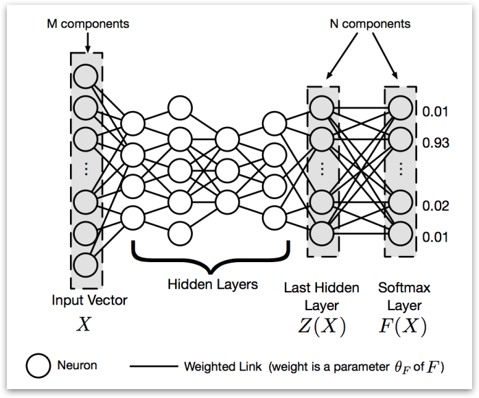
Neural networks typically produce class probabilities by using a “softmax” output layer that converts the logit, \(z_i\), computed for each class into a probability, \(q_i\), by comparing \(z_i\) with the other logits.
$$ q_i = \frac{\exp(z_i/T)}{\sum_j exp(z_j/T)} $$
where \(T\) is a temperature that is normally set to 1. Using a higher value for \(T\) produces a softer probability distribution over classes.
In the simplest form of distillation, knowledge is transferred to the distilled model by training it on a transfer set and using a soft target distribution for each case in the transfer set that is produced by using the cumbersome model with a high temperature in its softmax. The same high temperature is used when training the distilled model, but after it has been trained it uses a temperature of 1. It could reduce the computing resources required to run a network, allowing usage on a smaller scale like in embedded chips and IoT devices.
How does Distillation Work?
-
A Deep Neural Network(DNN) is trained with a high temperature, the \(T\) we mentioned before. The training of this first DNN is a high temperature because the high temperature forces the DNN to produce probability vectors with relatively large values for each class. The high temperature of a softmax is, the more ambiguous its probability distribution will be. The smaller the temperature of a softmax is, the more discrete its probability distribution will be.
-
A second Deep Neural Network is trained by replacing the hard labels of the training set with class probabilities output by the first Deep Neural Network.
Softmax Function under distillation
Softmax function is the Last layer of network. It’s used to normalize the outputs of the second to last layer. Under distillation situation, it has a parameter temperature (\(T\)). To perform distillation in softmax layer, a large network whose output layer is softmax is first trained on the original dataset. The softmax layer is a layer that considers a vector \(Z(X)\) of outputs produced by the last hidden layer of a DNN. Then we normalizes them into a probability vector \(F(X)\), the output of DNN assigning a probability to each class of dataset for input \(X\). \(T\) means temperature and shared across the softmax layer. (See the paper for the equations for \(F(X)\).)
Using Distillation as a Defense
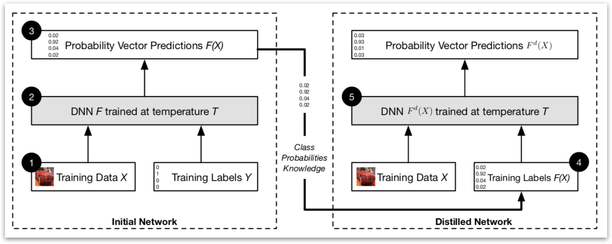
In distillation as a defense, the same network architecture is used in the distilled DNN as in the original DNN. First, this paper trained an initial network \(F\) on data \(X\) with a softmax temperature of \(T\).
Then, this paper uses the probability vector \(F(X)\), which includes additional knowledge about classes compared to a class label, predicted by network \(F\) to train a distilled network at temperature \(T\) on the same data \(X\).
Results
This paper evaluated Resilience, Sensitivity and Robustness on 2 datasets: MNIST and CIFAR10
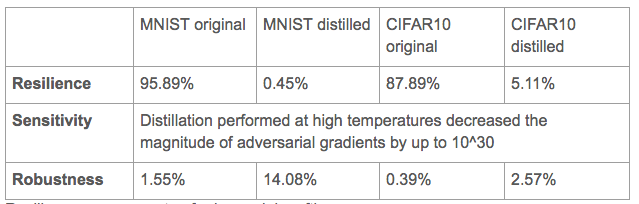
This paper also evaluated effect of Temperature on Adversarial Success Success of adversarial samples when changing at most 112 features.
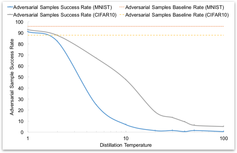
These results seem promising, but subsequent work found that Defensive Distillation is not actually robust to adversarial examples.
Why Distillation Seems to Work
First some attacks use the gradient of the logits, where softmax do not work here. Second, big difference in relative impact of changes in input to the softmax layer. Third, training at temperature \(T\) effectively increases all inputs to the softmax layer by a factor of \(T\), for example, Undistilled logits with Mean of 5.8/std of 6.4 and Distilled logits (T=100) with Mean of 482/std of 457.
Breaking Distillation
Instead of using the gradient of the input to the softmax layer, the gradient of the output of the softmax layer was used.Due to the problem of vanishing gradients, artificially divide the inputs to the softmax by \(T\). This method achieves a successful misclassification rate of 96.4%.
Towards Evaluating the Robustness of Neural Networks
Carlini, Nicholas, and David Wagner. Towards evaluating the robustness of neural networks. IEEE Symposium on Security and Privacy (“Oakland”) 2017. [PDF]
Carlini et al. proposed an optimization based attack to break the distillation defense mechanism developed by Papernot et al and other undistilled networks. This poses severe security problems to machine learning classifiers as the current defense strategy becomes vulnerable to this new type of strong white-box attacks. The attack is based on optimization approach, where the problem is formulated as
$$ \text{minimize}~\mathcal{D}(x,x+\delta) + cf(x+\delta)\\ \text{such that:}~x+ \delta \in [0,1]^{n} $$
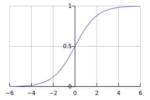
where \(f(x+\delta) \leq 0\) iff the classification result of \((x+\delta)\) is in class \(t\) (i.e. \(C(x+\delta) = t)\). \(c\) is a coefficient controling the relative importance of misclassification and norm minimization. Intuitive understanding of the optimization problem above is, we want a smaller perturbation (unobservable by human) by minimizing the norm \(||\delta||\) and causing misclassification by minimizing the function \(f(x+\delta)\). The constraint of \(x+\delta \in [0,1]^{n}\) is because this attack is conducted in image domain and has to generate valid images whose pixel value is in \([0,1]\) range. In order to further avoid the constraint, the authors apply \(tanh\) function to change the variables. Specifically, \(\delta_i = \frac{1}{2}(tanh(w_i)+1)-x_i \) and we directly optimize the unconstrained variable \(w_i \) instead of \(\delta_i\). ADAM is deployed to solve the above unconstrained optimization problem. A special note is the author implemented different \(p\)-norms \((p = 0, 2, \infty)\) under the optimization framework described above.
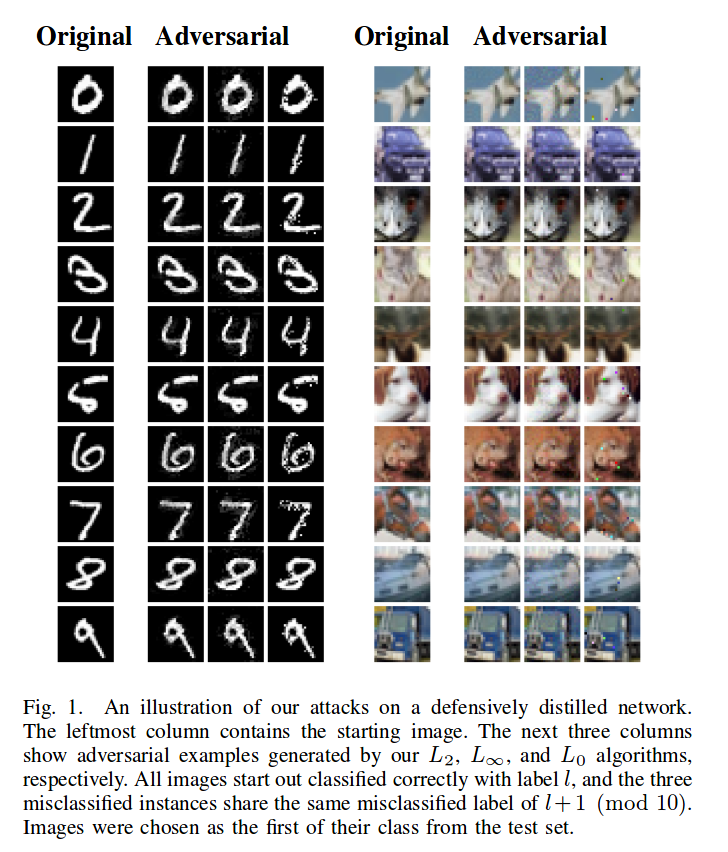
The evaluation part is compared to other existing white-box attack methods. Specifically, Fast Gradient Sign (FGS), Iterative Fast Gradient Sign (IFGS) methods are suitable for \(L_\infty \)-norm, Deepfool method is suitable for \(L_2\)-norm attack, JSMA method is suitable for \(L_0\)-norm attack. The target model for the listed attacks are distillation based network (defensitive strategy proposed for defending against FGS and IFGS methods) and normally trained neural networks. The final evaluation results demonstrate that the attack proposed in this work is far stronger than existing attack method in that it achieves highest attack success rate (this method achieves \(100%\) success rate while other methods don’t) and lowest perturbation magnitude. Some sample images generated from this attack are shown below. This attack is also now broadly accepted as a standard baseline for evaluating newly proposed defense mechanisms.
Obfuscated Gradients
Athalye, A., Carlini, N., & Wagner, D. “Obfuscated Gradients Give a False Sense of Security: Circumventing Defenses to Adversarial Examples.” ArXiv e-prints, arXiv: 1802.00420. February 2018.
Optimization-based attacks such as the Basic Iterative Method, Projected Gradient Descent, and Carlini and Wagner’s attack are powerful threat to most defenses against adversarial examples in machine learning classifiers. New defenses have been proposed that appear to be resistant to optimization-based attacks, but Athalye, Carlini, and Wagner argue that these defenses are not as robust as they claim.
Optimization-based attacks generate adversarial examples using gradients obtained through backpropagation. The authors identify obfuscated gradients as an element of many defenses that provides a facade of security by causing the attacker’s gradient descent to fail. Obfuscated gradients come in at least three forms: shattered gradients, stochastic gradients, and vanishing/exploding gradients.
A defense uses shattered gradients when it introduces non-differentiable operations, numeric instability, or otherwise causes the attacker’s gradient signal to be incorrect. A defense uses stochastic gradients when the inputs to the classifier are randomized or a stochastic classifier is used, resulting in a different gradient each time it is evaluated. Vanishing/exploding gradients are issues encountered in training some networks in which the gradient grows or shrinks exponentially during backpropagation. Some defenses involve multiple iterations of neural network evaluation. This can be viewed as evaluating one very deep neural network, which obfuscates the gradient signal by forcing the vanishing/exploding gradient problem.
Detecting Obfuscated Gradients
The authors propose a number of tests that might help detect when a defense relies on obfuscated gradients.
- Iterative attacks should work better than single-step attacks, since iterative attacks are strictly stronger than single-step attacks.
- White-box attacks should perform better than black-box attacks, since the black-box threat model is a strict subset of the white-box threat model.
- Attacks with an unbounded distortion metric (e.g. \(L_2\) norm) should find adversarial examples with 100% success.
- Optimization-based attacks should perform better than brute-force sampling of nearby inputs (sampling within an \(\epsilon\)-ball).
These tests may not cover all cases of obfuscated gradients, but they indicate when intuitive properties start to break down. All defenses with obfuscated gradients discussed by the authors fail at least one test.
Attack Techniques
The authors introduce attack techniques to address each of the three types of obfuscated gradients.
Shattered gradients can be attacked using a technique called Backward Pass Differentiable Approximation. For a classifier \(f(\cdot)\), some defenses make gradients unavailable to attackers by incorporating a non-differentiable preprocessing step \(g(\cdot)\), making the secured classifier \(\hat{f}(\cdot) = f(g(\cdot))\). Backward Pass Differentiable Approximation estimates gradients by substituting a smooth, differentiable approximation of \(g\).
Stochastic gradient-based defenses that randomly transform inputs can be defeated using the Expectation over Transformation technique to compute the gradient over the expected transformation of the input. If a stochastic classifier is used, the gradient can be similarly computed over the expectation of random parameters.
Defenses that use vanishing/exploding gradients can be circumvented by reparameterizing the secured classifier and optimizing over a space where vanishing/exploding gradients do not occur.
Seven of the eight defense techniques accepted to ICLR 2018 are based on a form of obfuscated gradients, and are therefore vulnerable to these attacks. The defense by Madry, et al., discussed below, was the only approach evaluated that doesn’t cause obfuscated gradients. Athalye, Carlini, and Wagner recommend that future defenses should be presented with specific, realistic threat models, testable claims with bounded test parameters, and evaluations against new defense-aware attacks.
Resistance to Adversarial Attacks
Aleksander Madry, Aleksandar Makelov, Ludwig Schmidt, Dimitris Tsipras, and Adrian Vladu. Towards Deep Learning Models Resistant to Adversarial Attacks. ICLR 2018. [PDF]
Madry et al. propose a general framework to study the defense of deep learning models against adversarial attacks. The goal of their framework is to provide precise security guarantees about how a particular defense stacks up against entire classes of attacks. Specifically, they offer the following saddle point problem:
$$\underset{\theta}{\text{min}} , \rho(\theta), \quad \text{where} \quad \rho(\theta) = \mathbb{E}_{(x, y) \sim \mathcal{D}} \bigg[ \underset{\delta \in \mathcal{S}}{\text{max}} , L(\theta, x + \delta, y) \bigg] , .$$
Let’s break this down:
- \( \theta \) is the set of parameters of the model. The attacker aims to exploit an existing model with a predetermined \( \theta \), and the defender can tune \( \theta \) as they wish.
- \( x \) and \( y \) are the example and label.
- \( L \) is the loss function.
- \( \mathbb{E} \) is a risk function.
This is a classic saddle point problem, consisting of two connected parts: an inner maximization problem, and an outer minimization problem. An adversary seeks to find an example that maximizes the model’s loss (the inner problem), and the defender seeks to tune their model such that the potential loss is minimized (the outer problem). Therefore, solving this problem (by minimizing rho) maximizes the robustness of a deep learning model.
The inner loss function was modeled with a fast gradient sign method (FGSM) attack. The FGSM perturbed data was used for as training data on the defense side. The outer minimization function was a little more complicated. It’s not simple enough to train on FGSM adversaries. We want something that’s universally robust, so we use PGD, a first-order method to solve constrained optimization problems. The authors used PGD to find local maxima, since they are the areas of highest loss.
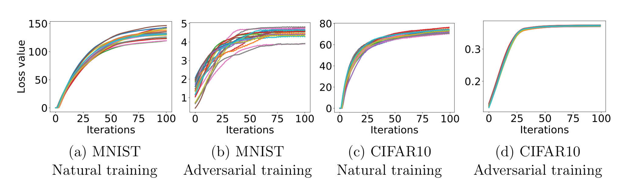
These graphs show how the loss scales as the number of PGD iterations increases. The loss grows and plateaus as the number of iterations grows (as expected for any model). However, the adversarially-trained models display much less loss than the naturally-trained models, indicating that Madry et. al.’s defense works well against their attacks.
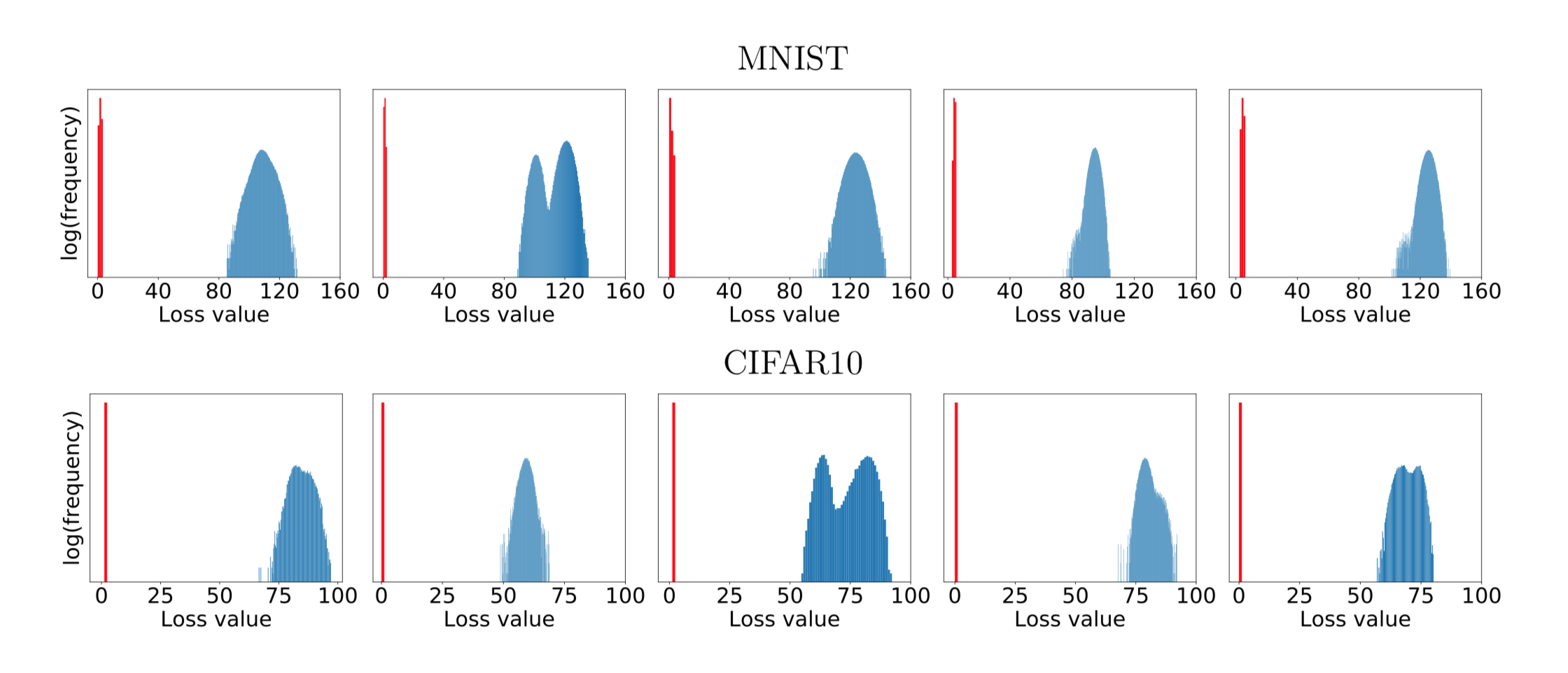
These graphs show the distributions of loss values, for various starting points. The loss values are obtained by randomly sampling points within an \(L\infty\)-ball centered at the starting point, then using PGD to find the local maxima near those random points. Although the locations of the points are widely distributed, the loss values are all clustered together. The authors claim that these graphs display the universality of PGD: any local maxima with significantly higher losses would likely be infeasible for any other first-order method to find.
— Team Gibbon: \
Austin Chen, Jin Ding, Ethan Lowman, Aditi Narvekar, Suya
References
[1] Carlini N, Wagner D. Towards evaluating the robustness of neural networks. InSecurity and Privacy (SP), 2017 IEEE Symposium on 2017 May 22 (pp. 39-57). IEEE.\
[2] Kingma DP, Ba J. Adam: A method for stochastic optimization. arXiv preprint arXiv:1412.6980. 2014 Dec 22.
[3] Goodfellow IJ, Shlens J, Szegedy C. Explaining and harnessing adversarial examples. arXiv preprint arXiv:1412.6572. 2014 Dec 20.
[4] Kurakin A, Goodfellow I, Bengio S. Adversarial examples in the physical world. arXiv preprint arXiv:1607.02533. 2016 Jul 8.
[5] Moosavi Dezfooli SM, Fawzi A, Frossard P. Deepfool: a simple and accurate method to fool deep neural networks. InProceedings of 2016 IEEE Conference on Computer Vision and Pattern Recognition (CVPR) 2016 (No. EPFL-CONF-218057).
[6] Papernot N, McDaniel P, Jha S, Fredrikson M, Celik ZB, Swami A. The limitations of deep learning in adversarial settings. InSecurity and Privacy (EuroS&P), 2016 IEEE European Symposium on 2016 Mar 21 (pp. 372-387). IEEE.
[7] Papernot N, McDaniel P, Wu X, Jha S, Swami A. Distillation as a defense to adversarial perturbations against deep neural networks. InSecurity and Privacy (SP), 2016 IEEE Symposium on 2016 May 22 (pp. 582-597). IEEE.
[8] A. Madry, A. Makelov, L. Schmidt, D. Tsipras, A. Vladu, “Towards Deep Learning Models Resistant to Adversarial Attacks”. February 2018.