Security and Privacy of Machine Learning

Class 3: Adversarial Machine Learning
Team Gibbon — 9 Feb 2018

This week’s topic covered some proposed adversarial example attacks and defenses. The underlying problem is that machine learning techniques assume that training and testing data are generated from the same distribution. Therefore, adversaries can choose inputs to exploit the algorithms by manipulating data. We began class by discussing common distance metrics, \(L_0, L_2\), and \(L\infty\), popular benchmarking datasets, and the history of adversarial ML. However, the main theme was defense techniques can be used safely to prevent adversarial attacks. Below we discuss four papers that discuss both effective and ineffective defenses.

Distillation as a Defense

Nicolas Papernot and Patrick D. McDaniel, Xi Wu, Somesh Jha, and Ananthram Swami. Distillation as a Defense to Adversarial Perturbations against Deep Neural Networks. IEEE Symposium on Security and Privacy, 2016. [PDF]

What is Distillation

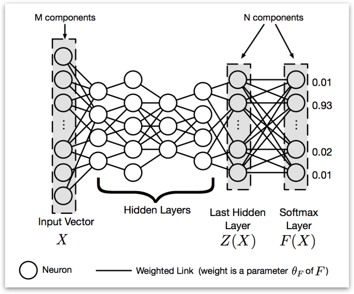
Neural networks typically produce class probabilities by using a “softmax” output layer that converts the logit, \(z_i\), computed for each class into a probability, \(q_i\), by comparing \(z_i\) with the other logits.

$$ q_i = \frac{\exp(z_i/T)}{\sum_j exp(z_j/T)} $$

where \(T\) is a temperature that is normally set to 1. Using a higher value for \(T\) produces a softer probability distribution over classes.

In the simplest form of distillation, knowledge is transferred to the distilled model by training it on a transfer set and using a soft target distribution for each case in the transfer set that is produced by using the cumbersome model with a high temperature in its softmax. The same high temperature is used when training the distilled model, but after it has been trained it uses a temperature of 1. It could reduce the computing resources required to run a network, allowing usage on a smaller scale like in embedded chips and IoT devices.

How does Distillation Work?

1. A Deep Neural Network(DNN) is trained with a high temperature, the \(T\) we mentioned before. The training of this first DNN is a high temperature because the high temperature forces the DNN to produce probability vectors with relatively large values for each class. The high temperature of a softmax is, the more ambiguous its probability distribution will be. The smaller the temperature of a softmax is, the more discrete its probability distribution will be.

2. A second Deep Neural Network is trained by replacing the hard labels of the training set with class probabilities output by the first Deep Neural Network.

Softmax Function under distillation

Softmax function is the Last layer of network. It’s used to normalize the outputs of the second to last layer. Under distillation situation, it has a parameter temperature (\(T\)). To perform distillation in softmax layer, a large network whose output layer is softmax is first trained on the original dataset. The softmax layer is a layer that considers a vector \(Z(X)\) of outputs produced by the last hidden layer of a DNN. Then we normalizes them into a probability vector \(F(X)\), the output of DNN assigning a probability to each class of dataset for input \(X\). \(T\) means temperature and shared across the softmax layer. (See the paper for the equations for \(F(X)\).)

Using Distillation as a Defense

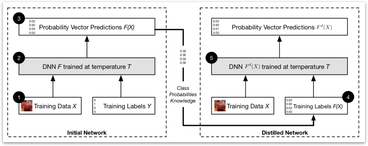
In distillation as a defense, the same network architecture is used in the distilled DNN as in the original DNN. First, this paper trained an initial network \(F\) on data \(X\) with a softmax temperature of \(T\).

Then, this paper uses the probability vector \(F(X)\), which includes additional knowledge about classes compared to a class label, predicted by network \(F\) to train a distilled network at temperature \(T\) on the same data \(X\).

Results

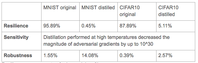
This paper evaluated Resilience, Sensitivity and Robustness on 2 datasets: MNIST and CIFAR10

This paper also evaluated effect of Temperature on Adversarial Success Success of adversarial samples when changing at most 112 features.

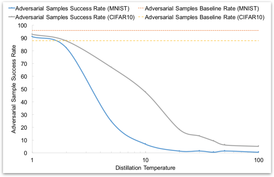
These results seem promising, but subsequent work found that Defensive Distillation is not actually robust to adversarial examples.

Why Distillation Seems to Work

First some attacks use the gradient of the logits, where softmax do not work here. Second, big difference in relative impact of changes in input to the softmax layer. Third, training at temperature \(T\) effectively increases all inputs to the softmax layer by a factor of \(T\), for example, Undistilled logits with Mean of 5.8/std of 6.4 and Distilled logits (T=100) with Mean of 482/std of 457.

Breaking Distillation

Instead of using the gradient of the input to the softmax layer, the gradient of the output of the softmax layer was used.Due to the problem of vanishing gradients, artificially divide the inputs to the softmax by \(T\). This method achieves a successful misclassification rate of 96.4%.

Towards Evaluating the Robustness of Neural Networks

Carlini, Nicholas, and David Wagner. Towards evaluating the robustness of neural networks. IEEE Symposium on Security and Privacy (“Oakland”) 2017. [PDF]

Carlini et al. proposed an optimization based attack to break the distillation defense mechanism developed by Papernot et al and other undistilled networks. This poses severe security problems to machine learning classifiers as the current defense strategy becomes vulnerable to this new type of strong white-box attacks. The attack is based on optimization approach, where the problem is formulated as

$$ \text{minimize}~\mathcal{D}(x,x+\delta) + cf(x+\delta)\\ \text{such that:}~x+ \delta \in [0,1]^{n} $$

where \(f(x+\delta) \leq 0\) iff the classification result of \((x+\delta)\) is in class \(t\) (i.e. \(C(x+\delta) = t)\). \(c\) is a coefficient controling the relative importance of misclassification and norm minimization. Intuitive understanding of the optimization problem above is, we want a smaller perturbation (unobservable by human) by minimizing the norm \(||\delta||\) and causing misclassification by minimizing the function \(f(x+\delta)\). The constraint of \(x+\delta \in [0,1]^{n}\) is because this attack is conducted in image domain and has to generate valid images whose pixel value is in \([0,1]\) range. In order to further avoid the constraint, the authors apply \(tanh\) function to change the variables. Specifically, \(\delta_i = \frac{1}{2}(tanh(w_i)+1)-x_i \) and we directly optimize the unconstrained variable \(w_i \) instead of \(\delta_i\). ADAM is deployed to solve the above unconstrained optimization problem. A special note is the author implemented different \(p\)-norms \((p = 0, 2, \infty)\) under the optimization framework described above.

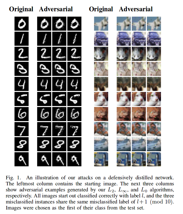
The evaluation part is compared to other existing white-box attack methods. Specifically, Fast Gradient Sign (FGS), Iterative Fast Gradient Sign (IFGS) methods are suitable for \(L_\infty \)-norm, Deepfool method is suitable for \(L_2\)-norm attack, JSMA method is suitable for \(L_0\)-norm attack. The target model for the listed attacks are distillation based network (defensitive strategy proposed for defending against FGS and IFGS methods) and normally trained neural networks. The final evaluation results demonstrate that the attack proposed in this work is far stronger than existing attack method in that it achieves highest attack success rate (this method achieves \(100%\) success rate while other methods don’t) and lowest perturbation magnitude. Some sample images generated from this attack are shown below. This attack is also now broadly accepted as a standard baseline for evaluating newly proposed defense mechanisms.

Obfuscated Gradients

Athalye, A., Carlini, N., & Wagner, D. “Obfuscated Gradients Give a False Sense of Security: Circumventing Defenses to Adversarial Examples.” ArXiv e-prints, arXiv: 1802.00420. February 2018.

Optimization-based attacks such as the Basic Iterative Method, Projected Gradient Descent, and Carlini and Wagner’s attack are powerful threat to most defenses against adversarial examples in machine learning classifiers. New defenses have been proposed that appear to be resistant to optimization-based attacks, but Athalye, Carlini, and Wagner argue that these defenses are not as robust as they claim.

Optimization-based attacks generate adversarial examples using gradients obtained through backpropagation. The authors identify obfuscated gradients as an element of many defenses that provides a facade of security by causing the attacker’s gradient descent to fail. Obfuscated gradients come in at least three forms: shattered gradients, stochastic gradients, and vanishing/exploding gradients.

A defense uses shattered gradients when it introduces non-differentiable operations, numeric instability, or otherwise causes the attacker’s gradient signal to be incorrect. A defense uses stochastic gradients when the inputs to the classifier are randomized or a stochastic classifier is used, resulting in a different gradient each time it is evaluated. Vanishing/exploding gradients are issues encountered in training some networks in which the gradient grows or shrinks exponentially during backpropagation. Some defenses involve multiple iterations of neural network evaluation. This can be viewed as evaluating one very deep neural network, which obfuscates the gradient signal by forcing the vanishing/exploding gradient problem.

Detecting Obfuscated Gradients

The authors propose a number of tests that might help detect when a defense relies on obfuscated gradients.

• Iterative attacks should work better than single-step attacks, since iterative attacks are strictly stronger than single-step attacks.
• White-box attacks should perform better than black-box attacks, since the black-box threat model is a strict subset of the white-box threat model.
• Attacks with an unbounded distortion metric (e.g. \(L_2\) norm) should find adversarial examples with 100% success.
• Optimization-based attacks should perform better than brute-force sampling of nearby inputs (sampling within an \(\epsilon\)-ball).

These tests may not cover all cases of obfuscated gradients, but they indicate when intuitive properties start to break down. All defenses with obfuscated gradients discussed by the authors fail at least one test.

Attack Techniques

The authors introduce attack techniques to address each of the three types of obfuscated gradients.

Shattered gradients can be attacked using a technique called Backward Pass Differentiable Approximation. For a classifier \(f(\cdot)\), some defenses make gradients unavailable to attackers by incorporating a non-differentiable preprocessing step \(g(\cdot)\), making the secured classifier \(\hat{f}(\cdot) = f(g(\cdot))\). Backward Pass Differentiable Approximation estimates gradients by substituting a smooth, differentiable approximation of \(g\).

Stochastic gradient-based defenses that randomly transform inputs can be defeated using the Expectation over Transformation technique to compute the gradient over the expected transformation of the input. If a stochastic classifier is used, the gradient can be similarly computed over the expectation of random parameters.

Defenses that use vanishing/exploding gradients can be circumvented by reparameterizing the secured classifier and optimizing over a space where vanishing/exploding gradients do not occur.

Seven of the eight defense techniques accepted to ICLR 2018 are based on a form of obfuscated gradients, and are therefore vulnerable to these attacks. The defense by Madry, et al., discussed below, was the only approach evaluated that doesn’t cause obfuscated gradients. Athalye, Carlini, and Wagner recommend that future defenses should be presented with specific, realistic threat models, testable claims with bounded test parameters, and evaluations against new defense-aware attacks.

Resistance to Adversarial Attacks

Aleksander Madry, Aleksandar Makelov, Ludwig Schmidt, Dimitris Tsipras, and Adrian Vladu. Towards Deep Learning Models Resistant to Adversarial Attacks. ICLR 2018. [PDF]

Madry et al. propose a general framework to study the defense of deep learning models against adversarial attacks. The goal of their framework is to provide precise security guarantees about how a particular defense stacks up against entire classes of attacks. Specifically, they offer the following saddle point problem:

$$\underset{\theta}{\text{min}} , \rho(\theta), \quad \text{where} \quad \rho(\theta) = \mathbb{E}_{(x, y) \sim \mathcal{D}} \bigg[ \underset{\delta \in \mathcal{S}}{\text{max}} , L(\theta, x + \delta, y) \bigg] , .$$

Let’s break this down:

• \( \theta \) is the set of parameters of the model. The attacker aims to exploit an existing model with a predetermined \( \theta \), and the defender can tune \( \theta \) as they wish.
• \( x \) and \( y \) are the example and label.
• \( L \) is the loss function.
• \( \mathbb{E} \) is a risk function.

This is a classic saddle point problem, consisting of two connected parts: an inner maximization problem, and an outer minimization problem. An adversary seeks to find an example that maximizes the model’s loss (the inner problem), and the defender seeks to tune their model such that the potential loss is minimized (the outer problem). Therefore, solving this problem (by minimizing rho) maximizes the robustness of a deep learning model.

The inner loss function was modeled with a fast gradient sign method (FGSM) attack. The FGSM perturbed data was used for as training data on the defense side. The outer minimization function was a little more complicated. It’s not simple enough to train on FGSM adversaries. We want something that’s universally robust, so we use PGD, a first-order method to solve constrained optimization problems. The authors used PGD to find local maxima, since they are the areas of highest loss.

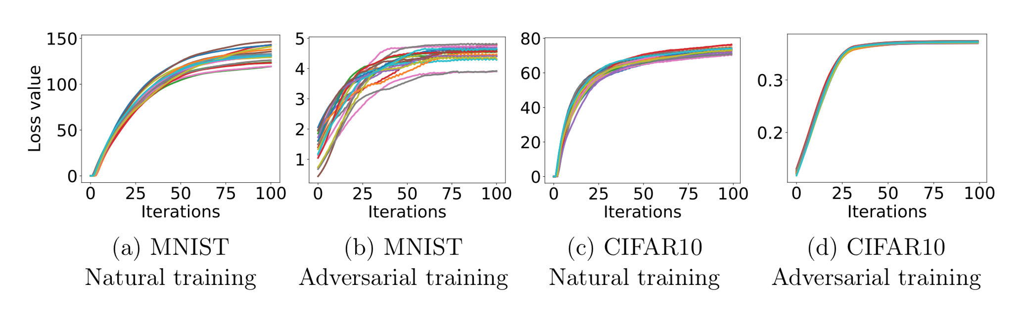
These graphs show how the loss scales as the number of PGD iterations increases. The loss grows and plateaus as the number of iterations grows (as expected for any model). However, the adversarially-trained models display much less loss than the naturally-trained models, indicating that Madry et. al.’s defense works well against their attacks.

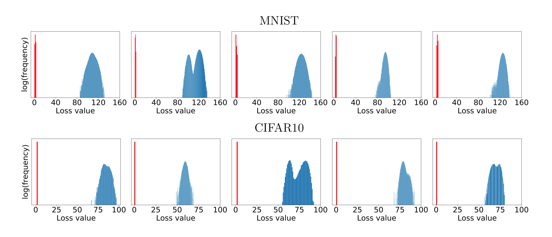
These graphs show the distributions of loss values, for various starting points. The loss values are obtained by randomly sampling points within an \(L\infty\)-ball centered at the starting point, then using PGD to find the local maxima near those random points. Although the locations of the points are widely distributed, the loss values are all clustered together. The authors claim that these graphs display the universality of PGD: any local maxima with significantly higher losses would likely be infeasible for any other first-order method to find.

— Team Gibbon: \
Austin Chen, Jin Ding, Ethan Lowman, Aditi Narvekar, Suya

References

[1] Carlini N, Wagner D. Towards evaluating the robustness of neural networks. InSecurity and Privacy (SP), 2017 IEEE Symposium on 2017 May 22 (pp. 39-57). IEEE.\

[2] Kingma DP, Ba J. Adam: A method for stochastic optimization. arXiv preprint arXiv:1412.6980. 2014 Dec 22.

[3] Goodfellow IJ, Shlens J, Szegedy C. Explaining and harnessing adversarial examples. arXiv preprint arXiv:1412.6572. 2014 Dec 20.

[4] Kurakin A, Goodfellow I, Bengio S. Adversarial examples in the physical world. arXiv preprint arXiv:1607.02533. 2016 Jul 8.

[5] Moosavi Dezfooli SM, Fawzi A, Frossard P. Deepfool: a simple and accurate method to fool deep neural networks. InProceedings of 2016 IEEE Conference on Computer Vision and Pattern Recognition (CVPR) 2016 (No. EPFL-CONF-218057).

[6] Papernot N, McDaniel P, Jha S, Fredrikson M, Celik ZB, Swami A. The limitations of deep learning in adversarial settings. InSecurity and Privacy (EuroS&P), 2016 IEEE European Symposium on 2016 Mar 21 (pp. 372-387). IEEE.

[7] Papernot N, McDaniel P, Wu X, Jha S, Swami A. Distillation as a defense to adversarial perturbations against deep neural networks. InSecurity and Privacy (SP), 2016 IEEE Symposium on 2016 May 22 (pp. 582-597). IEEE.

[8] A. Madry, A. Makelov, L. Schmidt, D. Tsipras, A. Vladu, “Towards Deep Learning Models Resistant to Adversarial Attacks”. February 2018.

Class 2: Privacy in Machine Learning
Team Nematode — 2 Feb 2018

In today’s post we introduce some key concepts crucial to understanding the current state of privacy in machine learning. In a time where novel machine learning applications are seemingly announced weekly, privacy is becoming more relevant as learning algorithms play varied and sometimes critical roles in our lives. We introduce differential privacy and common ‘solutions’ that fail to protect individual privacy, explore membership inference attacks on blackbox machine learning models, and discuss a case study involving privacy in the field of pharmacogenetics, where machine learning models are used to guide patient treatment.

Membership inference attacks

Reza Shokri, Marco Stronati, Congzheng Song, and Vitaly Shmatikov. Membership Inference Attacks Against Machine Learning Models. IEEE Symposium on Security and Privacy (“Oakland”) 2017. [PDF]

Shokri et al. attempt to attack black box machine learning models based on subtle data leaks based on the outputs. If the membership of a datapoint can be identified in the training set of a black box machine, it poses a significant privacy risk to the data of users of machine learning services. This is especially important for machine learning services such as Google Prediction and Amazon ML, as an inability to guarantee the privacy of training data would preclude a significant number of customers from using their services.

The attack is based on the idea that there are noticeable patterns in outputs when the input is given to the model as training data. While no human would be able to pick up on a pattern of that nature, a machine learning model with a theoretically limitless data source has that power. As the purpose of machine learning is to notice and evaluate patterns beyond human recognition, using a machine learning model to attack black box machine learning models makes sense.

For a machine learning model to attack the black box, it first needs to train against other models where it can verify its own accuracy. For this, similar models need to be created for evaluation. These models are called shadow models, and need to be trained on similar sample data to the original model. To generate training data, these models use hill climbing methods on the black box to seek high confidence areas. By then sampling data using a simple distribution about those points, somewhat accurate training sets can be created. Ideally, these sets will be roughly the same size and distribution of the target model.

The attack model is then trained on a set of shadow models, using classifications based on whether or not the datapoint was in the training set of the shadow model. This theoretically works based on the attack model being able to locate areas in which the curves are overfitted in the shadow models and translate that into membership. Ultimately, the study produced results that ranged from 70% to 95% precision overall based on the target model. The model gave nearly no false negatives.

To limit the power of these attacks, more regularization can be used to minimize overfitting, as the overfitting patterns become less apparent as the curve fitting is minimized. However, differential privacy is the more general class of solutions that is the defining foundation of the current state of the field of privacy in machine learning.

Differential privacy

With the explosion of data collection from various social platforms and the increasing usage of machine learning on personalized applications like personalized medication, medical diagnostics, genomics and face recognition, the collection of sensitive human data is inevitable. When dealing with personal information, it is paramount to preserve the privacy of any individual participating in the data set. In a word, it is necessary to ensure that an adversary does not learn about the presence or absence of any individual’s information from looking at the synopsis of the data set. This goal is the central motivation the concept of differential privacy.

To fully appreciate differential privacy, let us discuss some alternative solutions to preserving individual privacy in a data set identify how each one fails in achieving the goal of privacy.

Failed alternatives

1. Allowing only group queries

It seems intuitive that individual data privacy can be preserved by restricting a user to only group queries. For example, a group query can be: “How many students in this class earned an A?”. But this blatantly violates the privacy if the user also queries “How many students in this class apart from Rick earned an A?”, where the end user can know if Rick received an A or not based on the answer to the two queries.

2. Add random noise to the query result

Adding random noise to the query result tends to obfuscate the relation between the input and the output, but an adversary can determine the noise distribution by repeated querying. Hence, this approach also fails.

3. Deterministic perturbation in answering

We can deterministically map every output to another value in the vector space to obfuscate the input-output relation. But this becomes far too computationally complex in a high-dimensional regime.

4. Withholding sensitive information

An easy, straightforward notion is to simply withhold any sensitive data before executing any query; however, this very action reveals information about the presence or absence of sensitive data.

5. Make output independent of any individual record

This approach certainly does not reveal the presence or absence of an individual in the data set. But this method is not of any practical use since, by mathematical induction, the output does not depend on the data set itself.

6. K-anonymity

Another way to achieve obfuscation of a record is to group it with \(k\) other records for each attribute. Unfortunately, this method also fails in high-dimensional cases, where it has been shown to be feasible to still distinguish an individual record.

7. Semantic Security

Semantic security is a strict notion in cryptography which ensures that the advantage of an adversary with an auxiliary information should be cryptographically small with or without the access to the output (ciphertext). In our query model, this definition is too strong and does not allow learning any useful information from the data set.

Defining differential privacy

The formal definition of differential privacy is given as:

A randomized computation \(M\) satisfies \(\epsilon\)-differential privacy if for any adjacent data sets \(x\) and \(x’\), and any subset \(C\) of possible outcomes \(Range(M)\),

$$Pr[M(x) \in C] \leq \exp(\epsilon) \times Pr[M(x’) \in C]$$

In other words, this means that the chance that an event occurs with your data and the chance it would occur without your data is closely bounded by a privacy budget \(\epsilon\). The figure below depicts the equation where the two lines denote the probability distribution over \(x\) and \(x’\).

There is another relaxed version of the above definition of differential privacy, called \((\epsilon,\delta)\)-differential privacy, defined as below:

A randomized computation \(M\) satisfies \((\epsilon,\delta)\)-differential privacy if for any adjacent data sets \(x\) and \(x’\), and any subset \(C\) of possible outcomes \(Range(M)\),

$$Pr[M(x) \in C] \leq \exp(\epsilon) \times Pr[M(x’) \in C] + \delta$$

The above definition basically implies that with probability \((1-\delta)\), \(M\) preserves \(\epsilon\)-differential privacy.

Properties of differential privacy

Group Privacy: An \(\epsilon\)-differentially private algorithm can be extended to provide group privacy for a group size of \(k\) by scaling the privacy budget to \(k\epsilon\).

Composition: Composition of \(k \epsilon\)-differential privacy and \((\epsilon,\delta)\)-differential privacy methods leads to \(k \epsilon\)-differential privacy and \((k \epsilon, k \delta)\)-differential privacy methods respectively.

Differential privacy with Laplace noise

To ensure \(\epsilon\)-differential privacy for a function \(f(x)\), we can add Laplace noise to it:

$$ f(x) + \text{Laplace}(0, \sigma)^d $$

where \(\Delta f = \text{max} || f(x)-f(x’) ||_1 \) and \(\sigma \geq \frac{\Delta f}{\epsilon}\).

Let us consider a working example. Consider that there are two adjacent data sets \(D\) and \(D’\) consisting of scores of students of a class, such that \(D\) and \(D’\) differ by only one student’s record.

Consider the function \(f\) that computes the class average. If, say, the minimum and maximum attainable scores are \(0\) and \(100\) respectively, then the sensitivity of \(f\) is \( \frac{100-0}{4} = 25\).

Thus, to release the class average of \(D\) is given by \(\frac{65+83+77+56}{4}\) with \(\epsilon\)-differential privacy, we would add the result of sampling \(\text{Laplace}(0, \frac{25}{\epsilon})\) to the computed value. This preserves the privacy of the student differing in \(D\) and \(D’\).

Privacy in Pharmacogenetics

Matthew Fredrikson, Eric Lantz, Eric and Jha, Somesh and Lin, Simon and Page, David and Ristenpart, Thomas Privacy in Pharmacogenetics: An End-to-End Case Study of Personalized Warfarin Dosing. USENIX Security Symposium 2014. [PDF]

In their case study, Fredrikson et al. analyze personalized Warfarin doses, a widely used anticoagulant. Finding the correct dose of Warfarin is vitally important as both low and high doses may result in death of the patient – literally, a matter of life and death.

This experiment was done on the available IWPC dataset which contains and uses demographic information (age, height, weight, race), genetic markers (CYP2C9/VKORC1) and clinical histories of people around the world to predict their appropriate Warfarin dose. The IWPC has found that linear regression is the best learning model to fit the data and has made the model available for physicians’ use in calculating the initial dose of the Warfarin.

Let’s highlight how an adversary can use model inversion attack to violate the genomic privacy of a patient. We first initially assume that an adversary has black-box access to the trained model. As it turns out, due to the highly linear nature of the data, by running the model backwards, the sensitive genotype can be predicted given the stable dose of Warfarin, some basic demographic facts regarding the patient, and the marginal priors of the patient distribution.

How does the attack work? First, the adversary computes all the values of the missing variables that could potentially agree with the given information. Then, the adversary runs the model forward for each hypothetical patient in the dataset to predict the stable Warfarin doses. Finally, the adversary performs a likelihood computation to find out which configuration of the missing variables are most probable. Given the information and model inversion setting, this algorithm is optimal, as it minimizes the adversaries misprediction rate. With respect to the baseline, the accuracy of the model inversion attack is only 5% lower in comparison to ideal prediction.

As seen in this image, the attacker computes the values of missing variables, then predicts the Warfarin doses; and finally, using this information, finds the most likely configuration.

Adding noise using differential privacy strategy can be a countermeasure against the model inversion attack. But using differential privacy decreases the utility of the trained model. Based on their simulated trials, authors claim that there is no such privacy budget that can prevent model inversion, without introducing risk of overfixed dosing.

The Netflix Prize: Semi-supervised deep learning from private training data

Frank McSherry and Ilya Mironov, Differentially Private Recommender Systems: Building Privacy into the Netflix Prize Contenders. KDD 2009. [PDF]

Traditional recommender systems are usually not designed with an emphasis on privacy, which can be detrimental when the adversary are able to create multiple accounts to affect the recommendation at will. Researchers have been successful in developing powerful attack linking records in the Netflix Prize data set with other public user data. The implication is that sensitive information as the input of a recommender system can be linked and made inference about. Similar practical examples include making inference about purchase history through Amazon’s recommendations.

McSherry and Mironov’s paper adapted the leading recommendation algorithms (factor models and neighborhood models) to the differential privacy framework in order to develop a recommender system based on the Netflix data set while providing privacy guarantees. As mentioned in the above section, differential privacy enables privacy preserving computation by substantially precluding inference from the output data, unlike the prior efforts focusing mainly on cryptographic solutions that limit access to data of users. By doing so, it is conceivable that more uncertainty/noise is added to computation.

One interesting aspect this paper dealt with is the privacy vs. accuracy tradeoff. Evaluation of their approach was applied to the Netflix Prize data set which bears extremely high dimensionality. The root mean squared error (RMSE) was used as the metric for accuracy. The findings are as the quality of privacy increases, the accuracy of the recommendation drops.

Privacy vs. accuracy over time was also studied to explore how the loss of accuracy due to privacy-preserving decreased as more data become available for a fixed value of the privacy parameter. The results are summarized in the following figure.

Conclusion

We have introduced differential privacy and formally defined what is meant by preservation of \(\epsilon\)-differential privacy; discussed common solutions and how they fail; explained the properties of a differentially private algorithm, and how adding Laplace Noise enables \(\epsilon\)-differential private functions. We also discussed how in Membership Inference Attacks Against Machine Learning Models, Shokri et al. discuss attacking a black box model by training on a set of shadow models. Finally, we discussed how in Privacy in Pharmacogenetics: An End-to-End Case Study of Personalized Warfarin Dosing Fredrikson et al. demonstrate how a model inversion attack can be employed to infer patient genotype information.

— Team Nematode: \
Bargav Jayaraman, Guy “Jack” Verrier, Joshua Holtzman, Max Naylor, Nan Yang, Tanmoy Sen

References

[1] R. Shokri, M. Stronati, C. Song, V. Shmatikov, “Membership Inference Attacks Against Machine Learning Models.” May 2017.

[2] M. Fredrikson, E. Lantz, S. Jha, S. Lin, D. Page, T. Ristenpart, “Privacy in Pharmacogenetics: An End-to-End Case Study of Personalized Warfarin Dosing.” August 2014.

[3] F. McSherry, I. Mironov, “Differentially Private Recommender Systems: Building Privacy into the Netflix Prize Contenders.” June 2009.

[4] A. Narayanan, V. Shmatikov, “Robust De-anonymization of Large Sparse Datasets.” May 2008.

[5] J. A. Calandrino, A. Kilzer, A. Narayanan, E. W. Felten, V. Shmatikov, “‘You Might Also Like’: Privacy Risks of Collaborative Filtering.” May 2011.

[6] C. Dwork, “Differential Privacy and Pan-Private Algorithms.” August 2016.

[7] C. Dwork, “Differential Privacy - Lecture 1”. August 2016.

Class 1: Intro to Adversarial Machine Learning
Team Panda — 26 Jan 2018

Machine Learning Background

In supervised Machine Learning, we train models with training data along with the label associated with it. We extract features from each sample, and use an algorithm to train a model where the inputs are those features and the output is the label.

For classifying the testing data, the classifier uses decision boundary to separate points of the data belonging to each class. In a statistical-classification problem with two classes, a decision boundary partitions all the underlying vector space into two separate classes. A support vector machine (SVM) is a linear classifier which constructs a boundary by focusing two closest points from different classes and it finds the line that is equidistant to these two points.

Loss Functions

A loss function define that how good a given model is at making predictions for a given scenario. It has its own curve and its own gradients. The slope of the curve indicates the appropriate way of updating the parameters to make the model more accurate in case of prediction. A frequently used loss function is the 0-1 loss function.

where \(I\) is the indicator notation. Hinge loss function is also popular in machine learning field. It provides a relatively tight, convex upper bound on the 0-1 indicator function. s

Gradient Descent

Gradient Descent is an optimization algorithm which is used to minimize cost function by iteratively moving the direction of the steepest descent. In machine learning, we use gradient descent to update the parameters (coefficients in Linear Regression and weight in neural networks) of our model.

In the figure, weight is slowly decreasing from the initial stage. \(J_{min}\) is the minimum value of the cost function which can be obtained by optimizing the algorithm.

Recently, there have been many successful applications of Deep Neural Networks (DNN) in the fields of information retrieval, computer vision, and speech recognition. Despite their potential, deep neural architectures, like all other machine learning approaches, are vulnerable to what are known as adversarial samples. These systems can be fooled by targeted manipulations which slightly modifying a real example to trick the model into “believing” that this modified sample belongs to an incorrect class with high confidence. To defend against these adversarial attacks, many researchers are exploring several directions including data augmentation, increasing model complexity, retraining, pre-processing, etc. Their main goal is to protect the model against adversarial manipulations by the attackers.

Applications and Vulnerabilities

To get a better idea of what security and privacy mean in a machine learning context, we highlight a few applications and examine the possible consequences of vulnerabilities in these domains.

One of the most commonly-discussed applications is in self-driving cars, which use machine learning algorithms for image recognition tasks, such as identifying traffic signs and road hazards. If an attacker were to cause an erroneous classification, e.g. mistaking a stop sign for a speed limit sign or missing a pedestrian in a crosswalk, both property and human lives would be in jeopardy. (Although luckily self-driving cars use a variety of other techniques to avoid collisions, including detailed maps and LIDAR, so are likely to not be directly vulnerable to image mis-classification attacks.)

Machine learning has also found a place in the medical world, being used to identify patterns and trends in patient histories that can be used for diagnoses, to recognize abnormalities in medical imaging, and even to evaluate the efficiency of a hospital’s workflow. The use of machine learning in healthcare introduces a new concern - how can patient data be effectively utilized for beneficial purposes, like predicting appropriate drug dosages, without compromising patient privacy?

There are numerous other uses of ML today (targeted advertising, fraud detection, malware detection, etc.) and each carries particular security and privacy concerns.

Adversarial Examples

In machine learning, an adversarial example is an input that has been manipulated so that the model returns a different, incorrect output. A classic adversarial example for image classification is from a paper by Goodfellow et al., which features a photo of a panda that was originally classified correctly, but is misclassified when carefully-crafted noise is added. The model classifies the new image as a gibbon, even though human eyes can easily see it is a panda.

As outlined in Biggio et al.‘s paper on the history of adversarial machine learning, adversarial examples were first described in 2004 in the context of email spam filters. At this time, Dalvi et al. and Lowd and Meek realized that slight modifications to spam emails allowed them to pass through the filters, without greatly affecting the content of the message. From this point, the field expanded to study the potential for adversarial examples in other realms, like machine-learning-based image and malware classification. The increased usage of deep learning techniques for object recognition led to a surge in interest around 2014, when Szegedy et al. showed that deep convolutional neural networks were also susceptible to adversarial examples. Since then, interest in this field has only continued to increase, with more and more papers published each year.

Classifying Attacks

Attacks can be categorized by many different characteristics, but are often referred to in terms of the attack method, the goal of the attack, and the adversary’s level of knowledge, as detailed in Papernot et al..

Attack Method

A poisoning attack is when the adversary adds carefully-crafted samples into the training data, thereby disrupting the learning process and manipulating the final trained model. An evasion attack occurs when a sample originally correctly classified into class A is manipulated and fed back into the model, now receiving an output that is not class A. A key difference between these two attacks is where each occurs in the ML pipeline: poisoning attacks occur before the training stage and evasion attacks occuring after training, during the testing stage.

Goal of Attack

The goal of the adversary is another way to categorize attacks, which in this case means whether or not there was a specific goal classification or not. Error-generic (also called untargeted) attacks aim to find a sample close to a given seed that is misclassified, but do not have a specific target output class. Error-specific (targeted) attacks deliberately change the seed sample’s classification from the original class A to a chosen class B.

Adversary Knowledge

The level of knowledge the adversary possesses generally falls into one of three loosely defined categories: black box, grey box, and white box attacks. Black box attacks assume the lowest level of adversary knowledge, generally only allowing the final classification to be known without any finer details about the model. On the other end of the spectrum, white box attacks assume that the attacker knows everything about the model, including the specific algorithm used, the feature set, the training data, etc. An attack by an adversary who knows more about the model than a black box but less than a white box is called a grey box attack, although the exact definition tends to vary.

Modern Machine Learning as a Potemkin village

The term “Potemkin village” describes a difference between appeance and reality. In a paper by Goodfellow, Shlens, and Szegdy, modern machine learning methods are described as building “a Potemkin village that works well on naturally occuring data, but is exposed as a fake when one visits points in space that do not have high probability in the data distribution.” The apparent fragility of deep neural networks has been particuarly exposed, as seen in the panda picture above.

The two-faced nature of machine learning models to be both fragile and robout from two different angles leads to concerns in the security of machine learning algorithms. High confidence in classifying adversarial examples poses a threat to the integrity of the model’s output.

Fast gradient sign method (FGSM)

Also the paper mentioned a method for generating adversarial examples. Fast gradient sign method maximizes the error between the ground truth classification of the sample and minimizes the error to the target classification. The method is effecitve is generating the best pixels to change to achieve a higher loss, essentially acting as a reverse optimization method. FGSM simply traverses the loss curve by moving in the opposite direction of the gradient loss.

As we discussed, the sign method in the FGSM is an approximation to the actual gradient. Although the most accurate method would use the true gradient, the sign of the gradient is taken for the sake efficiency: since \(\epsilon\) reflect the adversarial strength (the maximum size perturbation allowed), this represents taking the largest step possible in each dimension in the direction given by the gradient. (There are many variations on FGSM that we’ll discuss in later posts, including iterative versions where a sequence of smaller steps is used.) FGSM showcases the fragility of machine learning models especially through visualizations such as the panda example.

Adversarial training

Effects of nonlinearities

One criticism of deep neural networks is that their nonlinearity creates vulnerabilities that can be exploited by adversarial examples. As shown below, the mode function cuts through the data points linearly, while the function drawn by the neural network conforms more tightly to the training data points. This overfitting to training data creates pockets in which the class chosen by the function does not match the ground truth class value for a given data point.

Solutions

As a possible solution, Szegedy et al. proposed incorporating adversarial examples into the training data. Using various techniques to find the vulnerable pockets in the model, the authors were able to generate examples that would fall into those adversarial region. Adding those samples to the training data results in a new model that does not follow the original training points as closely, creating a smoother, more accurate function.

Using an adversarial regularizer is also a technique to limit overfitting and vulnerability to adversarial examples. Goodfellow et al. describes a technique using the fast gradient sign method mentioned above as a regularizer. Their method generates adversarial examples using the fast gradient sign method and then trains the model with the adversarial examples. By continually updating the adversarial examples to the model, the adversarial regions are minimized. In the paper, they were able to reduce the error rate on adversarial examples from 0.94% to 0.84% using this approach. In order to reduce this error further, they also increased the model size and introduced early stopping on adversarial validation set error. Using these additional techniques they were able to drop the error rate on adversarial examples based on the FGSM from 89.4% to 17.9%. A combination of techniques introduced in training can significantly decrease the vunerability to simple adversarial attacks.

Transferability of adversarial samples

As shown above, an adversarial sample can fool a machine-learned model to misclassify it with high confidence. In particular, the adversarial samples made to fool image classifiers show how an adversarial sample can be indistinguishable to humans from legitimate samples. Additionally, examples that evade one classifier tend to evade others. This poses a vulnerability for machine learned models, one that can be exploited with cross-evasion.

Learning classifier substitutes

For example, Papernot et al., took advantage of the transferability of adversarial examples on a remote DNN by training a new model with their own synthetic data. By using a relatively small number of queries to label their data, they trained a substitute model which they then used to craft adversarial samples. Demonstrating transferability, 84.24% of the adversarial samples trained from the substitute model fooled the remote DNN.

To explicitly demonstrate the phenomenon of both intra and cross-technique transferability, Papernot et al. used five different machine learning algorithms on five disjoint training sets of MNIST dataset. With this setup, adversarial samples trained from one technique on one subset of the training data fools – to varying degrees – models trained by a different subset of the training data as well as a different technique. Furthermore, an ensemble classifier could be fooled at a rate of up to 44%.

— Team Panda:
Christopher Geier, Faysal Hossain Shezan, Helen Simecek, Lawrence Hook, Nishant Jha

References

[1] I.J. Goodfellow, J. Shlens, C. Szegedy, “Explaining and Harnessing Adversarial Examples.” ArXiv e-prints, December 2014.

[2] B. Biggio, F. Roli, “Wild patterns: Ten years after the rise of adversarial machine learning.” arXiv preprint arXiv:1712.03141, 2017.

[3] N. Dalvi, P. Domingos, Mausam, S. Sanghai, D. Verma, “Adversarial classification,”” Int’l Conf. Knowl. Disc. and Data Mining, 2004, pp. 99–108.

[4] D. Lowd, C. Meek, “Adversarial learning,” Int’l Conf. Knowl. Disc. and Data Mining, ACM Press, Chicago, IL, USA, 2005, pp. 641–647.

[5] N. Papernot, P. McDaniel, A. Sinha, M. Wellman, “Towards the science of security and privacy in machine learning.” IEEE European Symposium on Security and Privacy, 2018.

[6] N. Papernot, P. Mcdaniel, I.J. Goodfellow, “Transferability in machine learning: from phenomena to black-box attacks using adversarial samples” arXiv preprint arXiv:1605.07277, 2016.

[7] C. Szegedy, W. Zaremba, I. Sutskever, J Bruna, D. Erhan, I.J. Goodfellow, R. Fergus. “Intriguing properties of neural networks.” ICLR, abs/1312.6199, 2014.

First Week
David Evans — 20 Jan 2018

This message was also sent out by email.

Since not everyone has joined the slack yet, I’m sending this out by email, but please make sure to join https://secprivml.slack.com soon. I will use that for future communications.

I have grouped the 18 full participants in the class into three teams of six:

Team Bus:

Anant Kharkar
Ashley Gao
Atallah Hezbor
Joshua Holtzman
Mainuddin Ahmad Jonas
Weilin Xu

Team Gibbon:

Aditi Narvekar
Austin Chen
Ethan Lowman
Guy “Jack” Verrier
Jialei Fu
Jin Ding

Team Panda:

Bargav Jayaraman
Christopher Geier
Faysal Hossain Shezan
Nathaniel Grevatt
Nishant Jha
Tanmoy Sen

The teams will probably adjust a bit over the next week as some people who registered for the class didn’t submit a survey, and others may be joining the class late, etc., but otherwise we will plan to keep with these teams through spring break and possible re-arrange things after that. You can, of course, rename your team and develop your own adversarial (but tasteful) team icon.

Each week, one team will be responsible for leading the class, one team for blogging (writing a summary of the class), and one team for food. Everyone in the class is expected to do the preparation for each meeting, which will usually involve reading a few papers (but may involve other activities, at the design of the leading team). See https://secml.github.io/teams/ for the description of team responsibilities. For the first week, Team Bus will be the leading team, Team Gibbon will be the feeding team, and Team Panda will be the blogging team. I have created a slack channel for each team, and you should have an invitation to join it. The immediate tasks for each team are:

• Team Bus: decide on a leader who will be responsible for coordinating your team for this week, come up with some ideas what you would like to do for Friday’s meeting, make sure there are some people who can come to my office hours on Monday (2:30pm) - if not enough people can come then, arrange an alternative time with me, and plan an exciting and worthwhile seminar for Friday.

• Team Gibbon: you are the feeding team for this week, so should select 2-3 people to take care of this. One of you should pick up a credit card from me on Thursday to pay for the food. You will be leading the seminar on 2 Feb, so should determine a leader for this, and once Team Bus posts the topic and paper for this week (which should happen on Monday), should start planning your topic. We should meet briefly after Friday’s seminar, to discuss your plans, and then a longer meeting the following Monday.

• Team Panda: you are the blogging team for this week, so should get familiar with https://secml.github.io/blogging/. You will be leading the seminar or 9 Feb, so should start thinking of topics you would like to lead. You should identify leaders for blogging, feeding, and leading to be ready for the next 3 weeks.

Cheers,

— Dave

Starting Seminar
David Evans — 15 Jan 2018

Our first seminar meeting will be Friday, January 26 (not this Friday, which would normally be the first class day, since I will be getting back from California too late to meet this week). Meetings will be Fridays in Rice 032, 9:30am-noon.

Since we’re missing the normal first meeting, I want to do as much of the organizational stuff this week to be able to have a substantive first meeting next week. This means we will group students into teams, have a team assigned to lead the first class, and announced topic and readings by next Tuesday (Jan 23).

To enable this, everyone interested in participating in the class in any way should:

1. Submit this form by Wednesday (Jan 24): https://goo.gl/forms/FqSmUNHYBPbaKsg72

2. Read the course syllabus, and follow the directions there to join the seminar slack group.

I will work out the teams based on the form submissions, and set up the schedule for leading classes/blogging. I will have office hours on Monday (Jan 22) at 2:30pm. People from the first presenting team will be expect to meet with me then (not necessarily everyone but at least some of the team), and anyone with questions about the seminar is also welcome to come by. (If this time works for the class, we’ll keep this as my regular office hours time for the semester.)

Sorry for missing the first class, but I think we’ll be able to manage most of what we would have done the first day electronically, and be able to have an effective first meeting on Jan 26.

Syllabus Posted
David Evans — 31 Dec 2017

The Syllabus is now posted.

Welcome
David Evans — 31 Dec 2017

This graduate-level special topics course will be offered in Spring 2018. Meetings will be Fridays, 9:30-noon in Rice Hall 032. More information will be posted here soon, but the seminar format will be roughly similar to what we used to TLSeminar last Spring.

This seminar will focus on understanding the risks adversaries pose to machine learning systems, and how to design more robust machine learning systems to mitigate those risks.

The seminar is open to ambitious undergraduate students (with instructor permission), and to graduate students interested in research in adversarial machine learning, privacy-preserving machine learning, fairness and transparency in machine learning, and other related topics. Previous background in machine learning and security is beneficial, but not required so long as you are willing and able to learn some foundational materials on your own. For more information, contact David Evans.

— 1 Jan 0001

Resources for Adversarial Machine Learning Research

Adversarial Machine Learning Toolkits

EvadeML-Zoo

cleverhans

Machine Learning Systems

Detectron - Facebook’s research platform for object detection research (including RetinaNet)

— 1 Jan 0001

See Teams for the class teams and responsibilities.

— 1 Jan 0001

Syllabus

cs6501: Security and Privacy of Machine Learning

University of Virginia, Spring 2018

Meetings: Fridays, 9:30AM - noon, Rice Hall 032

Course Objective. This seminar will focus on understanding the risks adversaries pose to machine learning systems, and how to design more robust machine learning systems to mitigate those risks.

Expected Background: Previous background in machine learning and security is beneficial, but not required so long as you are willing and able to learn some foundational materials on your own. Most students in the seminar should have either strong background in machine learning, or strong background in security and privacy, but it is not expected that most students have extensive background in both areas. The seminar is open to ambitious undergraduate students (with instructor permission), and to graduate students interested in research in adversarial machine learning, privacy-preserving machine learning, fairness and transparency in machine learning, and other related topics.

Coordinator: David Evans (evans@virginia.edu). My office is Rice 507.

Course Expectations

Students in the seminar are expected to:

• Lead discussions on interesting topics during the class meetings. For each week, there will be a team of students charged with preparing a topic and leading the discussion, and another team charged with writing a blog post about the class. Students responsible for posting the blog summary will be different from the ones charged with leading the topic discussion, but should work closely with the leaders on the posted write-up.

• Particpate actively in class meetings. This means being prepared to contribute by doing the assigned preparation (which will typically involve reading a few research papers, but may involve other things also) and thinking about the materials deeply to be able to contribute well to discussions.

• Contribute fully to a team that develops a course-long project which could either be a research project or a systematization of knowledge project. We will discuss this more in an early class, and form teams based on interests.

Communications

Course Website: https://secml.github.io/. All course materials will be posted on the course website, and students will be expected to provide materials to add to this site.

Slack: https://secprivml.slack.com. We will use a slack group for class communications. You can join using any @virginia.edu email address. You can also create slack channels for your team communications.

Honor and Responsibility

We believe strongly in the value of a community of trust, and expect all of the students in this class to contribute to strenghtening and enhancing that community. The course will be better for everyone if everyone can assume everyone else is trustworthy. The course staff starts with the assumption that all students at the university deserve to be trusted.

In this course, we will be learning about and exploring some vulnerabilities that could be used to compromise deployed systems. You are trusted to behave responsibility and ethically. You may not attack any system without permission of its owners, and may not use anything you learn in this class for evil. If you have any doubts about whether or not something you want to do is ethical and legal, you should check with the course instructor before proceeding.

Area Requirements

Note for CS Graduate Students. This course is mislisted in SIS (indeed, it is a “bug” in the setup of SIS that cannot be overcome that requires all grad courses to be assigned areas) as counting for the “Software Systems” and “Theory” area requirements. As per the actual rules in the Graduate Handbook, a cs6501 seminar course does not a priori count for any particular areas. It may be possible to count it for any area, but it would be up to you to make the case to your committee that it should count for a given area. In most cases, this will depend a lot on what you individually do in the class - for example, you could select presentation topics and a topic for you project that would make a strong case for counting it for the “Theory” area, but someone else who does a systems-focused project would be able to count it for a different area. I can help provide guidance on this, but it is ultimately up to your committee to decide if a course counts for a particular area requirement.